A Framework for Evaluating Intersection Collisions Involving Motorcycles - Part 2

Note: This post assumes that you have read the prior post.

A More Nuanced Example

We can make the example of the prior post more nuanced by incorporating the influence of eccentricity [1] and time-to-collision (TTC) [2] into our evaluation of the motorcyclist’s PRT. This will lead us to a different PRT for the motorcyclist in the left lane versus the motorcyclist in the right lane. For a motorcyclist that needs to respond to the left-turning vehicle, the eccentricity for the motorcyclist in the left lane will be in the range of 3-6 degrees. For the motorcyclist approaching in the right lane, the eccentricity will be in the range of 5-9 degrees. For a motorcyclist in the left lane who needs to respond with braking, the TTC when the left turn begins would be in the range of 1.5 to 3 seconds. For motorcyclists in the right lane who need to respond, the TTC would likely be in the 2.5 to 4 second range.

Table 1 lists average PRTs obtained from IDRR for this scenario using these ranges of eccentricity and TTCs. The values listed in parenthesis are the 85th percentile PRTs. The perception-response times in Table 1 are parsed by TTCs that are either less than or greater than 3 seconds. This is because this dividing line is used in IDRR. Two observations can be made based on the data in Table 1. First, the parsing of the data into TTCs less than or greater than 3 seconds creates a discontinuity in the data that may be too simplistic for analysis of some crashes. For example, this data suggests that, for an intruding vehicle turning from the next lane, approaching drivers have had an average PRT of 0.9 seconds if the TTC was 2.9 seconds, but 1.6 seconds if the TTC was 3.1 seconds, a 0.7 second difference in PRT for an insignificant change in TTC. For this illustration, the PRTs listed in Table 1 will be used without modification, but for evaluating some crashes, the relationship between TTC and PRT may need to be evaluated in a more nuanced fashion. This will be explored in a later post.

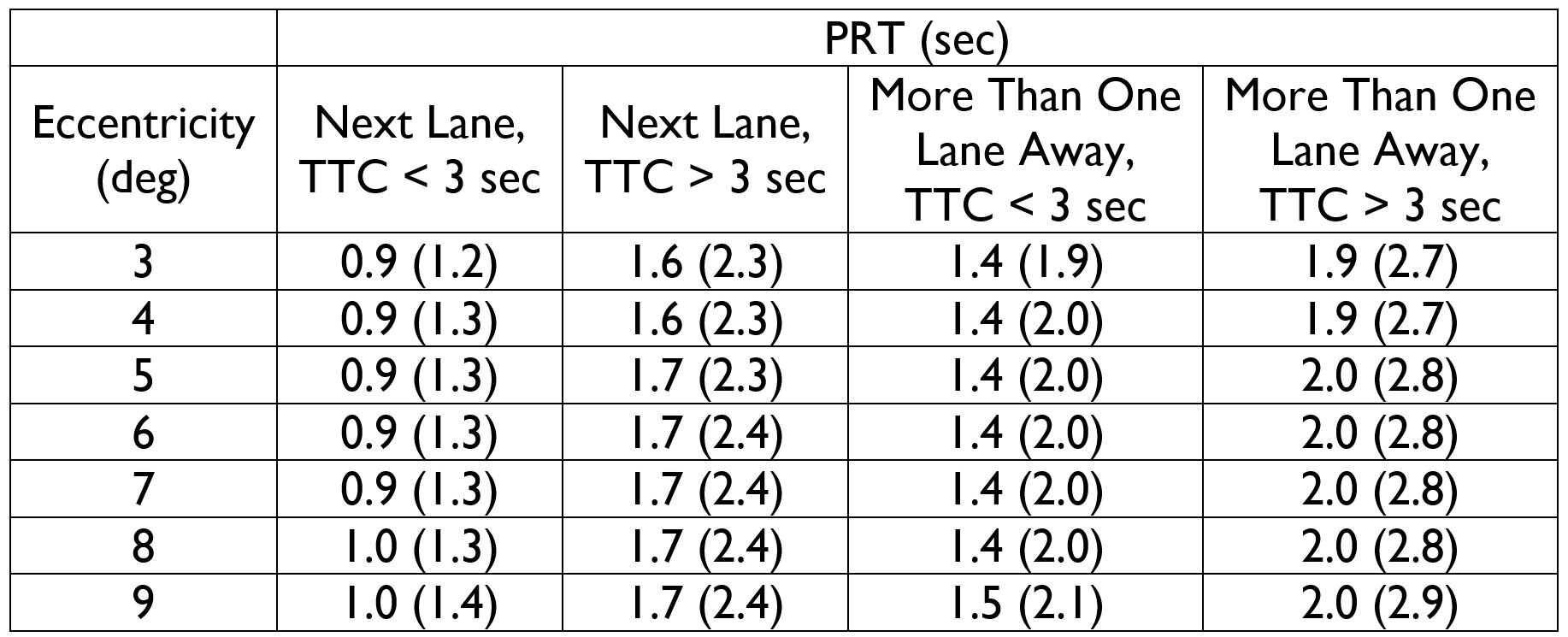
Table 1 – Perception-Response Times for LTAP-OD Scenarios from IDRR

Second, the PRTs for approaching drivers more than one lane away from the intruding driver are consistently longer than those for approaching drivers in the next lane. This seems to suggest that drivers or motorcyclists in the right lane would be using at least some of the additional time they have available to evaluate the situation – they are waiting, perhaps, until it becomes more clear (less ambiguous) what the left-turning driver is going to do.

An important question to be answered at this point is: When assessing a motorcyclist’s ability to avoid a crash, which perception-response time should be used – the average value or the 85th percentile (or, perhaps, a range of perception-response times could be used)? If we assume that for a population of drivers, the variability in perception-response times can be represented with normal distribution, then 50% of drivers will have a perception-response time faster than the average, and 50% of drivers will have a perception-response time slower than the average. To use the average perception-response time when assessing a motorcyclist’s or driver’s opportunity to avoid a hazard is to impose the assumption that a particular motorcyclist or driver will have a perception-response time faster than 50% of the population. There is typically no basis for such an assumption since there is physiological and psychological variation in the human population. Assuming a driver is not contributing to a slow reaction with inattention, distraction, or alcohol use, driver’s do not have control over where they fall within that natural variation.

Even for a single individual, their perception-response time could vary from occasion-to-occasion. There is, therefore, no basis for saying that the perception-response time of a motorcyclist who has a 75th percentile perception response time (for instance) is unreasonable. They are still within the spread of the population for normal, attentive motorcyclists. Beyond that physical and psychological reality, we as reconstructionists typically cannot know where a randomly selected motorcyclists (the motorcyclist involved in our crash) will fall within the population of motorcyclists when it comes to their perception-response time. Use of the average perception-response time would fail to acknowledge our uncertainty in this regard. While a randomly chosen motorcyclist could have a perception-response time as fast or faster than 50% of the population, the fair and conservative assumption is to assume they do not. For these reasons, when assessing the avoidability of a crash, it is more appropriate to use the 85th percentile perception-response time than to use the average [3].

Incorporating the 85th percentile PRTs from Table 1 into the example of the prior section results in the modified zones depicted in Figure 4. With different PRTs for the two motorcyclists, the benefit to a motorcyclist of being in the right lane is not as great as in the prior illustration, but it is still present. The red zone is still smaller in the right lane. The combined size of the yellow and gray zones (the area where braking by the motorcyclist makes a difference) is still smaller for the rider in the left lane compared to the rider in the right lane. Thus, the rider who chooses the right lane still benefits from increasing the lateral distance between themselves and the left turning vehicle. This would be reversed for a scenario where the Range Rover is attempting to cross the intersection from the motorcyclist’s right.

Figure 4 – Avoidance zones for this scenario (red = unavoidable; yellow = avoidable with a deceleration between 0.35 and 0.60 g; gray = avoidable with a deceleration between 0.00 and 0.35 g; brown = braking not necessary but might be employed and could result in a crash)

Endnotes

1. The eccentricity is the angle between the line defined by the motorcyclist’s approach direction and the line connecting the motorcyclist to the left-turning vehicle.

2. The time-to-collision is calculated from the instant the left turn begins (first lateral movement) until the time a collision would occur assuming the approaching driver did not brake.

3. This point is affirmed in the book Forensic Aspects of Driver Perception and Response, Fourth Edition, by David Krauss: “While they are undoubtedly useful and very commonly used, it is important to remember that the measures of central tendency [i.e., the average] represent but a single point in a distribution. They tell us nothing about the scatter in performance, the shape of the distribution, or how that distribution relates to other distributions that may be of interest. In addition, they are virtually no help in predicting what can be expected from one randomly selected individual…Accident investigators are generally interested in assessing the performance of a given individual, who is drawn from an unknown part of the distribution of interest. In such cases measures of central tendency are virtually useless as a guide…”